
NeuroImaging Methods
Functional neuroimaging data undergo multiple transformations from acquisition to interpretation. These transformations serve two main purposes: to remove noise and to facilitate interpretation. For example, fluctuations driven by neural activity account for only about 5% of the total signal. The remaining 95% consists of various sources of noise that must be addressed to prevent bias in results and interpretation — this is the “noise removal” part of the process.
Even after noise has been mitigated, functional neuroimaging data remain challenging to interpret due to their high dimensionality (a single scan may include minutes-long recordings across tens of thousands of brain locations) and the many unknowns surrounding brain function. Additional transformations and statistical analyses are therefore applied to render the data interpretable. In practice, extracting meaningful information from neuroimaging data often requires tools from basic statistics, machine learning, and graph theory.
I have contributed to both aspects of the functional neuroimaging analysis pipeline. My work on denoising has focused primarily on multi-echo fMRI. In terms of interpretation, I have leaded projects exploring dynamic (time-varying) functional connectivity and, on several occasions, delved into the world of dimensionality reduction using methods from machine learning (e.g., t-SNE, UMAP) and topological data analysis (e.g., the Mapper algorithm).
Please explore the sections below for more details.
 Multi-Echo fMRI
Functional MRI (fMRI) recordings capture not only fluctuations arising from localized neural activity but also from hardware instabilities, head motion, and physiological processes such as cardiac and respiratory cycles. As a result, fMRI practitioners dedicate considerable effort to isolating this informative component—both through improvements in acquisition protocols and the use of complex preprocessing pipelines. Multi-echo fMRI (ME-fMRI) represents a hybrid approach in which data are both acquired and processed differently.
In essence, ME-fMRI leverages the fact that BOLD effects—those associated with localized neural activity—depend linearly on echo time (an acquisition parameter defining the interval between excitation and signal readout), whereas non-BOLD fluctuations (e.g., motion or scanner instabilities) do not. By acquiring data simultaneously at multiple echo times (rather than a single one, as is typically done), researchers can identify signal components that exhibit the expected linear dependence and regress out the rest. Although ME-fMRI has existed for decades, it gained widespread adoption only recently, following the introduction of ME-ICA by the Bandettini lab (now implemented as tedana). ME-ICA combines echo-time–dependence analysis with independent component analysis to automatically remove non-BOLD fluctuations from fMRI data. While not perfect, tedana can markedly improve data quality, and many now view ME-fMRI as a key step toward enabling personalized mental healthcare interventions.
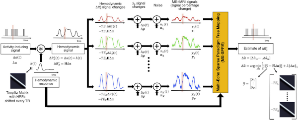
I have been an avid contributor to the ME-fMRI community since 2016. My work in ME-fMRI includes an early evaluation of the original ME-ICA approach, contributions to the tedana project (for example, I co-authored the first version of the dynamic report page during a hackathon), and devising, implementing and testing several iterations of a multi-echo–based deconvolution algorithm (see figure on the left). This last one in collaboration with my long-time friend Dr. Caballero-Gaudes at the Basque Center for Brain, Cognition and Language. For more details regarding my contributions to ME-fMRI, please check the references below.
If you’d like to learn more about ME-fMRI in general, I recommend this lecture linked below on the topic that I gave as part of an earlier version of the NIMH fMRI Summer Course.
Selected Publications on Multi-Echo fMRI:
- Gonzalez-Castillo J, et al. “Evaluation of Multi-Echo ICA denoising for task based fMRI studies: block designs, rapid event-related designs, and cardiac-gated fMRI” NeuroImage (2016)
- Caballero-Gaudes C, Moia S, Panwar PA, Bandettini PA, Gonzalez-Castillo J. “A deconvolution algorithm for multi-echo functional MRI: multi-echo sparse paradigm free mapping” NeuroImage (2019)
- DuPre et al. “TE-dependent analysis of multi-echo fMRI with tedana” Journal of Open Source Software (2021)
- Caballero-Gaudes C, Bandettini PA, Gonzalez-Castillo J. “A temporal deconvolution algorithm for multiecho functional MRI” IEEE 15th International Symposium on Biomedical Imaging (2018)
- Uruñuela E, Gonzalez-Castillo J et al. “Whole-brain multivariate hemodynamic deconvolution algorithm for functional MRI with stability selection” Medical Imaging Analysis (2024)
 Time-varying Functional Connectivity
What do neuroscientists mean when they talk about dynamic or time-varying functional connectivity? There’s quite a bit to unpack, and I am going to try my best to do so in a few paragraphs. That said, if you have the time and the interest, please check this talk before you keep going. It will all make much more sense after that!

Let’s start with functional connectivity (FC) itself. The term refers to the observation that groups of spatially non-contiguous brain regions—often referred to as brain networks—exhibit higher temporal synchrony with each other than with the rest of the brain. FC between two regions is typically measured using the Pearson’s Correlation between their respective time series. When this calculation is extended to hundreds of regions spanning the cortex (e.g., those defined by an atlas or parcellation), the result is a matrix of pairwise correlations known as a functional connectome.
A key point here is that these inter-regional correlations are computed using the entire duration of the scan. This makes sense—assuming the system is in a steady state, more data points yield more reliable correlation estimates.
But what if the system isn’t stationary? Is that “average” view of inter-regional relationships the whole story, or could additional insight be gained by examining how these connections fluctuate from second to second and minute to minute during a scan? While the static connectome has proven highly informative (as evidenced by thousands of studies), there may also be valuable information in these short-term, transient reconfigurations of brain connectivity. Understanding the meaning and potential clinical relevance of such time-varying functional connectivity remains an active and evolving area of research; one to which I have devoted many efforts.
In the early days, my work—like that of many others—focused on establishing the most basic aspects of dynamic functional connectivity (FC). In one of my first studies, we examined the spatial profile of FC dynamicity using hour-long resting-state scans (see more details here). Once we confirmed that FC fluctuations were spatially organized rather than random, I turned my attention to their potential cognitive correlates.
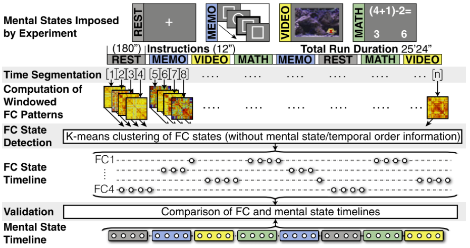
If dynamic reconfiguration of FC relates to cognition, then engaging in different mental activities should lead to corresponding changes in FC patterns. I demonstrated this in our 2015 PNAS publication, where participants were asked to mentally switch among four distinct mental activities while being continuously scanned during both engagement and transitions between them. The results confirmed that cognitive state changes indeed induce FC reconfigurations.
A key question, however, remained: what about the spontaneous reconfigurations observed during rest? Could these also reflect self-generated shifts in mental processes—the very essence of mind-wandering? I have devoted, and continue to devote, much of my work to exploring this fundamental question, which may hold clues to how the brain supports conscious experience. That inquiry belongs more squarely within the realm of cognitive neuroscience, so if you’re interested, you can read more about it here.
Alright, back to methods—since that’s the focus of this page. Let me highlight one purely methodological study I’ve conducted on time-varying FC. The first is a method comparison study led by my former mentee, Dr. Hua (Oliver) Xie, who was interested in identifying the most effective way to detect and characterize dynamic FC. This was no small task. Once the scientific community embraced the idea that time-varying FC might hold meaningful information, a proliferation of analytical methods emerged—ranging from various flavors of sliding-window correlation and dynamic conditional correlation (DCC) to multiplication of temporal derivatives and jackknife correlation, among others.
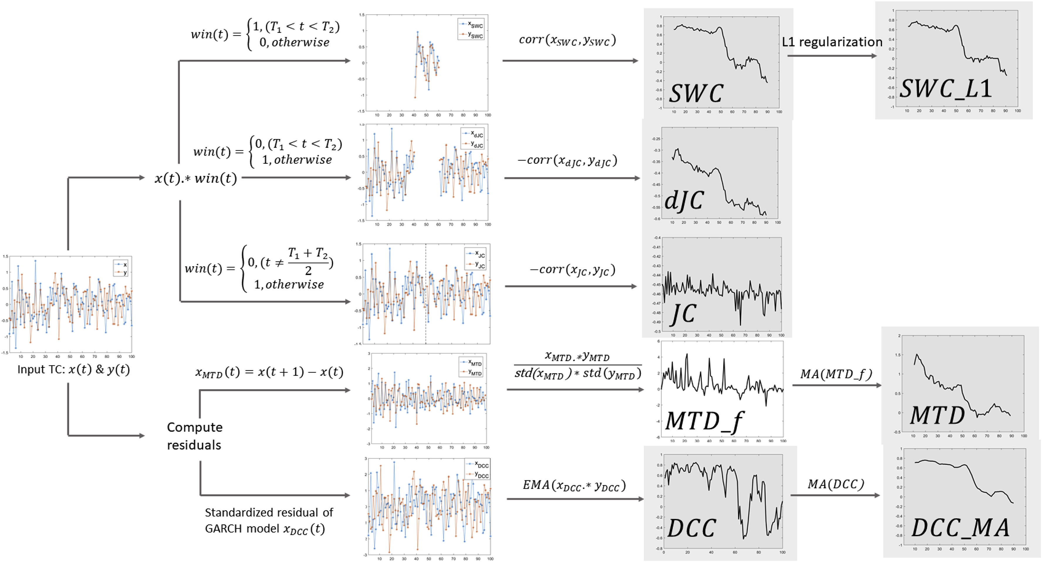
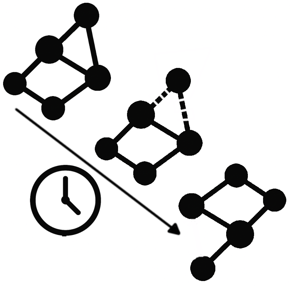
Oliver and I set out to compare seven of the most widely used methods for estimating time-varying FC (see figure on the right). We evaluated both their mathematical similarities and differences, as well as their practical performance in detecting FC reconfigurations linked to ongoing cognitive dynamics. For the latter, we relied on clustering analyses and evaluation metrics drawn from unsupervised machine learning.
Our results, reported here, showed that all window-based methods performed well for commonly used window lengths (WL ≥ 30 s), with the sliding-window methods (with and without normalization) and the hybrid dynamic conditional correlation with moving average (DCC_MA) approach performing slightly better. For shorter windows (WL ≤ 15 s), DCC_MA and jackknife correlation yielded the most robust results. These findings have since helped researchers make more informed choices about how best to characterize time-varying FC in their own studies.
Selected Publications on time-varying FC (methods-heavy):
Xie H et al. “Efficacy of different dynamic functional connectivity methods to capture cognitively relevant information” NeuroImage (2019)
Hutchinson et al. “Dynamic functional connectivity: promise, issues, and interpretations” NeuroImage (2013)
Gonzalez-Castillo J & Bandettini PA. “Task-based dynamic functional connectivity: Recent findings and open questions” NeuroImage (2018)
Xie et al. “Whole-brain connectiity dynamics reflect both task-specific and individual-specific modulation: a multitask study” NeuroImage (2018)
 Dimensionality Reduction
Humans are remarkably good at spotting patterns in up to three dimensions—perhaps a few more with the right tools. Think of color-coded movies of 3D scatter plots to visualize 5D data, radar charts and parallel coordinates to represent a handful of additional dimensions. But what happens when our data lives in 10,000+ dimensions, as in functional neuroimaging? Those tools fail unless we first project the data into a lower-dimensional space that preserves its essential structure.
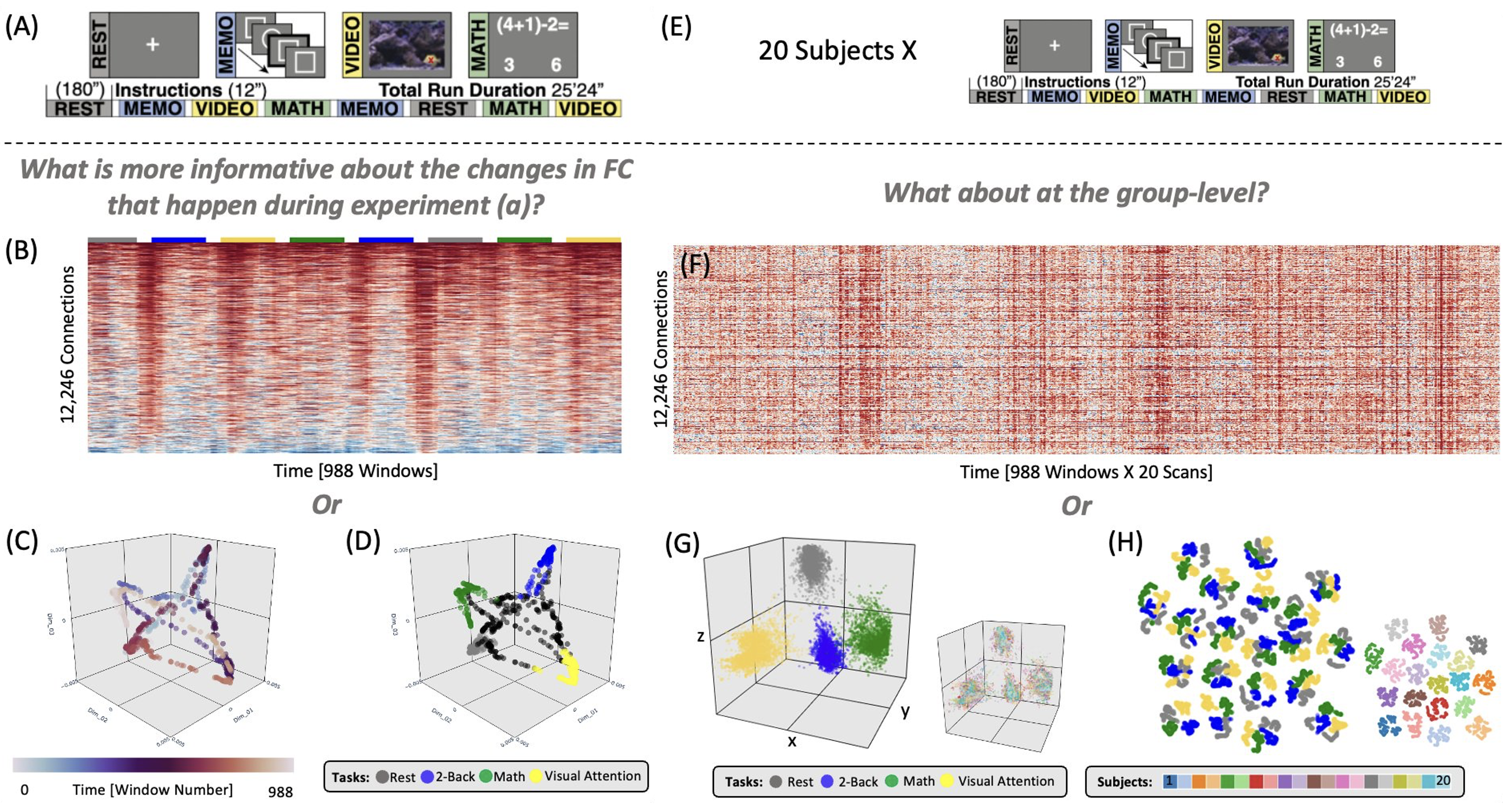
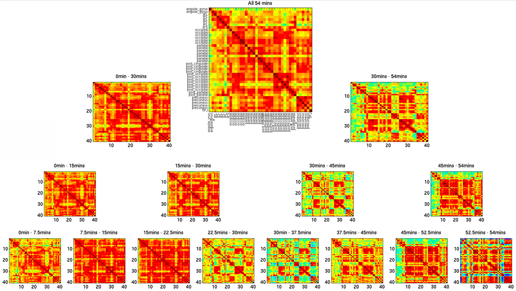
Take a concrete example from fMRI research. Suppose we record a 25-minute scan and parcellate the brain into 157 regions. To study how functional connectivity evolves over time, we can use a sliding-window correlation approach. The resulting matrix has 988 time points on the X-axis and 12,246 connections on the Y-axis (see left side of figure above). It essentially represents the evolution of data in a 12,246 dimensional space. Can you make sense of that directly? Probably not. But when we embed those data into three dimensions (panels C and D above), each dot now represents the connectivity pattern of a given time window, and clear structure emerges—four dominant configurations that recur at distinct times during the scan.
This example illustrates how high-dimensional data can be mapped into 2D or 3D while retaining meaningful information. Different dimensionality-reduction methods, however, make different assumptions. In a recent study, I compared three state-of-the-art nonlinear methods—t-SNE, UMAP, and Laplacian Eigenmaps—to evaluate how well they preserve information about subject identity and cognitive load in functional connectivity data. We found that all can work, but success depends critically on hyperparameter tuning. Importantly, heuristics from other fields do not necessarily apply here, underscoring the need for domain-specific exploration. Because many neuroimagers are new to these methods, the first part of our paper serves as a tutorial introduction. Check it out if you want to learn more on this topic! tions occured at two different instants of the scan. Want to know all the details, check this publication.
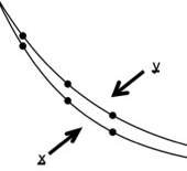
Another powerful approach to dimensionality reduction comes from Topological Data Analysis (TDA), particularly through the Mapper algorithm. I explored this method in collaboration with Dr. Manish Saggar from Stanford University, applying it to a multi-task fMRI dataset I had previously collected to study the cognitive relevance of time-varying functional connectivity. Unlike traditional sliding-window analyses, which collapse data over windows of ~30 seconds, TDA allowed us to capture the large-scale organization of whole-brain activity at the single-participant level without imposing arbitrary spatial or temporal averaging. The resulting low-dimensional representations (see example below) revealed both within- and between-task transitions at much finer time scales (~4–9 s). Moreover, individual differences in these dynamic trajectories predicted task performance.
These projects exemplify how I integrate advanced machine-learning approaches into neuroscience research. For more application-driven work using these and related methods, visit the section on neural correlates of conscious perception in Cognitive Neuroscience Research.